1. Structure Overview

The structure of the proposed visual SLAM estimator system is shown below:

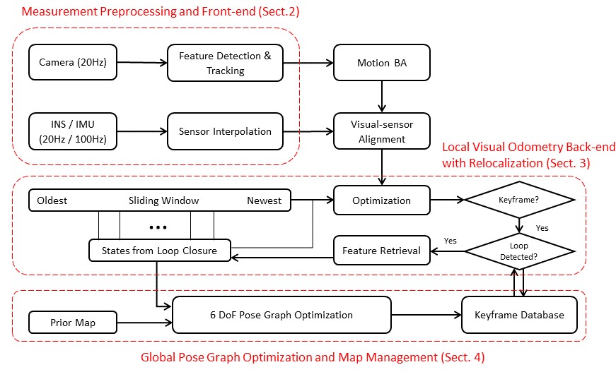
Fig. 1.1 Block diagram illustrates the full pipeline of our proposed stereo visual SLAM system (with INS assist). The system starts with measurement preprocessing (Section 2). The back end with relocalizatioin modules (see Section 3) tightly fuses INS measurements, feature observations, and redetected features from the loop closure. Finally, the pose graph module (with prior map loading) performs global optimization to eliminate drift.

1.1. Notations

We consider \((\cdot )^w\) as the world frame and \((\cdot)^b\) the body frame which we define as IMU/INS frame. \((\cdot)^c\) is the camera frame.

We use both rotation matrices \(\mathbf{R}\) and Halmilton quaternions \(\mathbf{q}\) to represent rotation. Primarily, quaternions are used in state vectors.

\(\mathbf{q}_b^w\) and \(\mathbf{p}_b^w\) are rotation and translation from the body frame to the world frame.

\(b_k\) is the body frame while taking the kth image. \(\otimes\) represents the multiplication operation between two quaternions.

For observed landmarks, we use \(\mathbf{p}_k^i\) as the \(i\) th 3D landmark point observed in the \(k\) th frame.

1.2. Formulation

VO (Visual Odometry) is the process of estimating the real-time location of the mobile camera. The only information available is the visual input from camera to observe the environment.

On top of visual odometry, visual SLAM (simultaneously localization and mapping) can be considered as a set of sub-tasks covering ego-motion estimation, as well as map representation, global bundle adjustment and loop closing. Each of them is an independent research topic and many methods have been proposed to solve one or some of them.

VIO (Visual Inertial Odometry) has the input from IMU/INS sensors apart from visual cues, classified into loosely-coupled and tightly-coupled types. In simple words, loosely-coupled model takes VO as a black box and fuses the output of VO and the input of IMU/INS to get a better estimation. On the other hand, tightly-coupled model takes IMU/INS data into the process of ego-motion and models the system differently. In our appliation, we choose the tightly-coupled model to acquire a more robust and accurate result.

In sum, the task of SSLAM Estimator is VO (Visual Odometry) / VIO (Visual Inertial Odometry) + Landmark Mapping + Loop Closure + Map Assisted Localization.

A process model that relates the robot pose at time \(k+1\) with the robot pose at time \(k\) can thus be described by

(1.1)\[\begin{equation} \mathbf{x}_k=f(\mathbf{x}_{k-1}, \mathbf{u}_k, \mathbf{w}_k)) \end{equation}\]

where \(\mathbf{u}_k\) is the control input at time \(k\) and \(\mathbf{w}_k\) is the process noise.

The observation model at time \(k\) is a function of \(\mathbf{x}_k\) and part of \(\mathbf{y}_j\) and is given by

(1.2)\[\begin{equation} \mathbf{z}_{k,j}=h(\mathbf{y}_j, \mathbf{x}_k, \mathbf{v}_{k,j}) \end{equation}\]

where \(\mathbf{v}_{k,j}\) is the observation noise at time \(k\). Note that the observation function is in general time-varying since only a subset of landmarks are observed at any given time stamp.

Influenced by noises, the poses \(\mathbf{x}\) and observations \(\mathbf{y}\) here denote random variables that obey some certain distribution, rather than fixed values. So we are trying to solve the problem of determining the distribution of the states given motion data \(\mathbf{u}\) and observation data \(\mathbf{z}\).

Actually under most cases, we reasonably assume the process noise and observation noise obey Gaussian distribution, so we only need to store the mean value and covariance matrix during each estimation. Therefore we convert state estimation problem into maximum likelihood (ML) problem by estimating the \(k\) time step state distribution according to the history data from \(0\) to \(k\):

\[\begin{equation} \label{equ.probability} P\left(\mathbf{x}_k | \mathbf{x}_0, \mathbf{u}_{1:k}, \mathbf{z}_{1:k} \right) \propto P\left( \mathbf{z}_k | \mathbf{x}_k \right)P\left(\mathbf{x}_k | \mathbf{x}_0, \mathbf{u}_{1:k}, \mathbf{z}_{1:k-1} \right) \end{equation}\]

where the first term is called likelihood and the second term is the prior probability.

\[\begin{equation} \label{equ.model} P\left(\mathbf{x}_k | \mathbf{x}_0, \mathbf{u}_{1:k}, \mathbf{z}_{1:k-1} \right) = \int P\left(\mathbf{x}_k | \mathbf{x}_{k-1}, \mathbf{x}_0, \mathbf{u}_{1:k}, \mathbf{z}_{1:k-1} \right) P\left(\mathbf{x}_{k-1} | \mathbf{x}_0, \mathbf{u}_{1:k}, \mathbf{z}_{1:k-1} \right) d\mathbf{x}_{k-1} \end{equation}\]

The traditional probabilistic filter based methods (including EKF and particle filter) assume the system follows the Markov property that the current $k$th state is only relevant to the previous :math:`(k-1)`th state. Then above equation can be simplified into:

(1.3)\[\begin{equation} P\left(\mathbf{x}_k | \mathbf{x}_0, \mathbf{u}_{1:k}, \mathbf{z}_{1:k-1} \right) = \int P\left(\mathbf{x}_k | \mathbf{x}_{k-1}, \mathbf{u}_{1:k} \right) P\left(\mathbf{x}_{k-1} | \mathbf{x}_0, \mathbf{u}_{1:k-1}, \mathbf{z}_{1:k-1} \right) d\mathbf{x}_{k-1} \end{equation}\]

Actually this model implies we only need to keep updating the state value \(\mathbf{x}\) by maintaining the mean value and covariance matrix, with the assumption that the states obey Gaussian distribution. The classic approach to solve this problem is to use EKF to obtain the maximum a posteriori (MAP) of the state value under linear approximation. As this report focuses on optimization based method, we skip the derivation of EKF solution.